 Weiner Advanced Development LLC
SQL at the limits of Big Data
Nearest date join
Another example of SQL standard practices that don't mesh well with the realities of Big Data is when joins are performed to create lots of possibilities and then “find” a special piece of information. Joining on “nearest date” fits this description.
If I have an accounts table that shows when customer accounts were started and my company runs many, short-run marketing campaigns to attract new customs. These campaigns overlap and are targeted at different customer segments. Since I expect the maximum new clients brought in by a campaign will be around the midpoint of the campaign, I want to assign likely-influenced-account-starts to each campaign based on closeness to the campaign midpoint and the customer is in the target market segment.
Now I have a data problem I can tackle - “assign each customer account start to the most likely influencing campaign”. We know the account start dates and the campaign midpoints with their target segment. The query just needs to join these two tables based on target segment and closest date.
No problem - I just need to find all the date differences and then select the closest. Typically this will look like:
select start_date, end_date, id, value, acct_type, promo_name, promo_peak_date
from (
    date, u.end_date, u.id, u.value, u.acct_type, p.promo_name, p.promo_peak_date,
    decode(u.start_date > p.promo_peak_date, true, u.start_date - p.promo_peak_date,
        p.promo_peak_date - u.start_date) as closeness,
    row_number() over (partition by id, start_date order by closeness, promo_peak_date ) closeness_order
from test_user_table u
left join promo_peaks p
  on u.acct_type = p.promo_acct_type )
where closeness_order = 1;
In this code we join our accounts with the promotion campaign information based only on the type (segment). This creates new information for all possible combinations of user account and promotion within a segment which can grow to a very large number of possibilities. In smaller datasets this growth is fine and can actually execute very quickly which is why this approach is common. However, when the dataset becomes very large this increase in row count created by the underqualified join makes so much data that the database struggles to process it. My favorite definition of Big Data is “data at the limits of current technology” and if your data is this large then creating massively more data is not a wise approach. This shows up as queries that “spill” (swap) to the disk drives or completely fills up disks with temp data crashing the query.
Below is the full test code used on a Redshift 1-node, dc2.large cluster, a small data warehouse but big enough to show the effect. The above query ran for 20 min and produced the expected results. When executing the disk storage of the cluster could be seen being consumed by temp data storage needed to execute the above query.
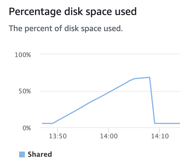
The query consumed over 60% of the total disk space on the cluster. An even slightly larger set of data would have consumed all available space leading to a “disk full” condition leading to, at least, a failure of the query.
Building on the previous whitepaper on this topic we can develop a better approach to this problem when dealing with Big Data and it starts with thinking about how I would manually perform this task if I was given 2 piles of index cards with data on them. I would lay them out, interdigitated, so that the campaign cards are in order with the account cards based on midpoint date for the former and start date for the latter. Then for each account card I would only need to look backwards and forwards for the nearest campaign card. The last step would be to select which is closer - the closest previous campaign or the closest later campaign. No new data need be created to perform this check.
The SQL for this process starts with UNIONing the tables together and then WINDOWing for the nearest campaign card of the right type. Lastly a selection of either the earlier closest or later closest campaign is made. The SQL for this process is:
with unioned as (
select promo_acct_type as acct_type, NULL as id, promo_name, promo_peak_date, NULL as start_date,
    NULL as end_date, NULL as value, promo_peak_date dt
from promo_peaks
union all
select acct_type, id, NULL as promo_name, NULL as promo_peak_date, start_date, end_date,
    value, start_date dt
from test_user_table)
,
combined as (
select *,
    NVL(max(promo_peak_date) OVER (partition by acct_type order by dt rows between unbounded preceding and
        1 preceding), '1970-01-01'::date) cb,
    NVL(min(promo_peak_date) OVER (partition by acct_type order by dt rows between 1 following and
        unbounded following), '2100-01-01'::date) ca
from unioned )
,
closest as (
select start_date, end_date, id, value, acct_type,
    case when coalesce(start_date - cb, 0) > (ca - start_date) then ca else cb end closest
from combined
where start_date is not NULL)
select c.start_date, c.end_date, c.id, c.value, c.acct_type, a.promo_name, a.promo_peak_date
from closest c
left join promo_peaks a
on c.closest = a.promo_peak_date and c.acct_type = a.promo_acct_type;
This approach to the problem results in a query that executes in 90 seconds and has zero spill to disk. The results from these two queries are exactly the same. This performance difference only gets larger when other activity is being done on the database (this test was done on an otherwise idle Redshift cluster). Memory demands and IO bandwidth demands from other queries running on an active database would far more greatly impact the first approach as it needs all the memory and all the disk IO bandwidth to execute in the measured 20 min. The revised query doesn’t have such high demands of the database.
This whitepaper and its companion show that when working with Big Data - Don’t Make More!
Test case code:
drop table if exists test_user_table;
create table test_user_table (
  start_date  date    encode zstd,
  end_date    date    encode zstd,
  id       int         encode zstd,
  value       float    encode zstd,
  acct_type   varchar(32) encode zstd
)
DISTKEY(acct_type)
SORTKEY(start_date, end_date);

insert into test_user_table (
with recursive twofivesix(n) as (
    select 0::int8 as n
    union all
    select n + 1
    from twofivesix t
    where n < 255
)
select decode(date_part('dw',start_date) in (0,6), true, start_date - 2, start_date)
        as start_date,  -- No weekend starts
    decode(date_part('dw',end_date) in (0,6), true, end_date + 2, end_date)
        as end_date,  -- No weekend ends
    id, value, acct_type
from (
    select   decode(start_date >= end_date, true, end_date - (random() * 90 + 1)::int, start_date )
            as start_date,  -- No starts after ends
        decode(end_date < current_date, true, end_date, NULL) as end_date,  -- No future ends
        id, value, acct_type
    from (
    select  current_date - ((random() * 1000)::int) as start_date,
            current_date - ((random() * 1000)::int - 90) as end_date,
            n as id, n::float / 7000000 as value, 'type-' || to_hex((n / 7) % 16) as acct_type
    FROM (select (a.n + b.n + c.n + d.n) as n from twofivesix a
        cross join (select n*256 as n from twofivesix) b
        cross join (select n*65536 as n from twofivesix) c
        cross join (select n*16777216 as n from ( select distinct (n/64)::int as n from twofivesix ) ) d
    )
    )
)
order by start_date, end_date
);
commit;

drop table if exists promo_peaks;
create table promo_peaks (
    promo_name    varchar(32) encode zstd,
    promo_peak_date    date encode zstd,
    promo_acct_type    varchar(32) encode zstd
)
DISTKEY (promo_acct_type)
SORTKEY (promo_peak_date);

insert into promo_peaks(
with recursive promo_dates(d, md) as
( select min(t.start_date) as d,
     max(t.start_date) as md
  from test_user_table t
    union all
    select d + 1 + ((random() * 5)::int) as d, md
    from promo_dates d
    where d.d <= d.md
    )
select 'promo-' || ((random() * 10000)::int)::text as promo_name,
            d as promo_peak_date,
      'type-' || to_hex((random() * 53)::int % 16) as promo_acct_type
from promo_dates
order by promo_peak_date );
commit;

end; vacuum test_user_table;
end; vacuum promo_peaks;
analyze test_user_table ;
analyze promo_peaks;
commit;


drop table if exists output1;
create temp table output1 as
with unioned as (
select promo_acct_type as acct_type, NULL as id, promo_name, promo_peak_date,  NULL as start_date,
    NULL as end_date, NULL as value, promo_peak_date dt
from promo_peaks
union all
select acct_type, id, NULL as promo_name, NULL as promo_peak_date, start_date, end_date,
    value, start_date dt
from test_user_table)
,
combined as (
select *,
    NVL(max(promo_peak_date) OVER (partition by acct_type order by dt rows between unbounded preceding
        and 1 preceding), '1970-01-01'::date) cb,
    NVL(min(promo_peak_date) OVER (partition by acct_type order by dt rows between 1 following
        and unbounded following), '2100-01-01'::date) ca
    --NVL(lag(promo_peak_date) IGNORE NULLS OVER (partition by acct_type order by dt),
        --'1970-01-01'::date) cb,
    --NVL(lead(promo_peak_date) IGNORE NULLS OVER (partition by acct_type order by dt),
        --'2100-01-01'::date) ca
from unioned )
,
closest as (
select start_date, end_date, id, value, acct_type,
  case when coalesce(start_date - cb, 0) > (ca - start_date) then ca else cb end closest
from combined
where start_date is not NULL)
select c.start_date, c.end_date, c.id, c.value, c.acct_type, a.promo_name, a.promo_peak_date
from closest c
left join promo_peaks a
on c.closest = a.promo_peak_date and c.acct_type = a.promo_acct_type
;
commit;

drop table if exists output2;
create temp table output2 as
select start_date, end_date, id, value, acct_type, promo_name, promo_peak_date
from (
    select u.start_date, u.end_date, u.id, u.value, u.acct_type, p.promo_name, p.promo_peak_date,
        decode(u.start_date > p.promo_peak_date, true, u.start_date - p.promo_peak_date,
        p.promo_peak_date - u.start_date) as closeness,
        row_number() over (partition by id, start_date order by closeness,
            promo_peak_date) as closeness_order
    from test_user_table u
    left join promo_peaks p
    on u.acct_type = p.promo_acct_type )
where closeness_order = 1
;
commit;

select count(*) from output1;
select count(*) from output2;

-- compare the output files
(select * from output1
except
select * from output2)
union all
(select * from output2
except
select * from output1)
;
PS. An interesting observation is that for Redshift “LAG … IGNORE NULLS OVER …” performed significantly worse than using “MAX … OVER”. This is likely due to the difficulty the optimizer has with the “ignore nulls” qualifier of the window function. The LAG() and LEAD() version of the query statements are included but commented out if others would like to explore this behavior.